Learning DataStructure (1): Hash Table

Introduction

What is Hash Table?

Hash table is a special form of an ordinary array. It can complete SEARCH, INSERT and DELETE in O(1) average time;

Core concepts

1. Hash Function and Collision;
2. Chaining and Open-Addressing;
3. Linear Probing and Double Probing;

Hash Function and Collision

Hash Function is used to compute the slot from the key k. Hash Function h map key k to a hash table
T [0, …, m - 1]:





We can understand by a simple example:

There is a teller h work in theater whose responsibility is to check each audience k’s ticket and arrange their seats. Several strategies are given:

1. List all seats before checking, in each check phrase h scan them from the head to find the first available one;
2. Each time after arranging k, h records the index of next available seat then arrange k + 1 on it;
3. h can initially push all seats in an array as index indicates, if a audience k in, the first seat will be kicked out;
4. Teller has a magic wand which can automatically arrange each k on a specific seat. No more operation needed;

Let’s take a closer look on these four strategies. The first one is linked list, every time you should search from head. Its time consumption increases progressively as consumers in. The second one is record a replica which will reduce the time complexity to O(1) but consumes more resources in recording this replica. The third one is stack which follows ‘first in, last out’ rule. The last one called ‘magic wand’ is hash table, which can find a specific seat without any plus operation;

The progress is simply showed as this picture:

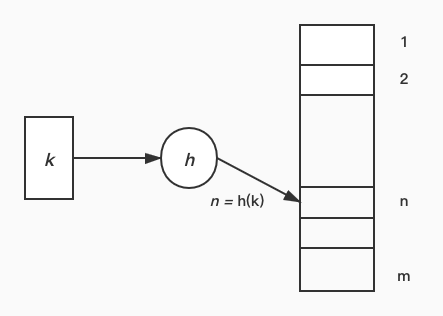
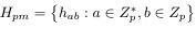
Such a progress is effective for small audience number, because all of them can be arranged on a unique position if h choose an ideal hash function. But when there are so many audience that no hash function work well to arrange them on unique position, collision will happen. So collision in hash progress defined that several keys will be mapped to a same slot.

After briefly introduce the definition of hash function and collision, we will discuss two most important things in this chapter:

1. How to choose an ideal hash function which can map each key k to an unique position in array as well as possible?
2. How to solve the collision effectively, namely, in time complexity and space complexity?

Choose a good hash function

If we wanna know what is a good hash function, we should know the criteria of a good hash function first:

Each key is equally likely to hash to any of the m slots, independently of where any other key has hashed to.

But unfortunately we have no way to check this condition. Fortunately, we have found a universal class of hash function. Let me give its mathematical definition first:

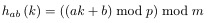
So for all a and b, if p and m is given, we can find a set contains all hash function:

such that:

You must want to ask: what is universal hash and what it can do?

We all know that collision will occur when hashing. If collision occurs, collision-solver (whatever it is) will be called. If n key map to one slot, the collision-solving’s time complexity will increase to O(n). Universal hashing aims to resolve this problem by randomly choosing hash function in a way that is independent of the keys that are actually going to be stored.

But actually, collision still exist for big data set. So we should apply collision-solver to tackle this problem. Two algorithms will be introduced: open-addressing and chaining

Chaining and Open-Addressing

Chaining

Chaining is to solve collision by storing all keys collide pairwise in a linked list which is as following picture:

Open-Addressing

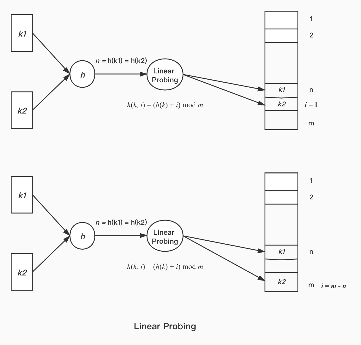
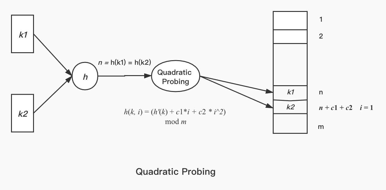
Open-Addressing is to solve collision by computing next position of the keys collided in a manner of probe. There are many probing algorithms, as we only introduce two commonly used:
Linear probing and Quadratic Probing; They work like following picture:

Load Factor

An important concept should be emphasized: load factor. The definition of load factor a is a = n/m such that n is the number of elements
and m is the size of hash table. Load factor represents the ratio between element’s number and hash table size. In practise, we almost predict the scale of usage to set the load factor (mostly we set m = 2^31).
We can infer from Calculus and Probability that the expected number of probes in a successful search is at most: 1/a ln(1/(1-a)). In Java Library, HashMap class sets the load factor 0.75.